These are a few notes on reproducibility. Based on a talk that I gave in a Research Seminar at Zucker Hillside Hospital in 2018 (the slides are here), I argue that we need to make our work reproducible to make it replicable. That is, reproducible for ourselves. Although replicability and reproducibility should be distinguished, the former depends on the latter. I identify three principles of making research reproducible: 1. Separating data from analysis; 2. using version control; 3. using code to analyze data. These three principles not only allow us to make our work reproducible; they also enable us to readily share our data and workflows with others. I introduce a working environment that is based on the editor emacs together with the outlining tool org-mode, the version control system git, and the statistical software R¹, all of which have a strong and supportive online community and are widely used by computer scientists and researchers across the world. They are ideal tools to make research reproducible.

To understand this difference, the following table by Kirstie Whitaker (see her excellent slides here) is very useful:

Thus, work is reproducible when identical code on identical data give identical results. Achieving this takes some effort; it's not reproducible if it only runs on your laptop. That said, there are a few steps that can be integrated into regular work flows that will make it at least more likely that our work is reproducible on other machines as well.

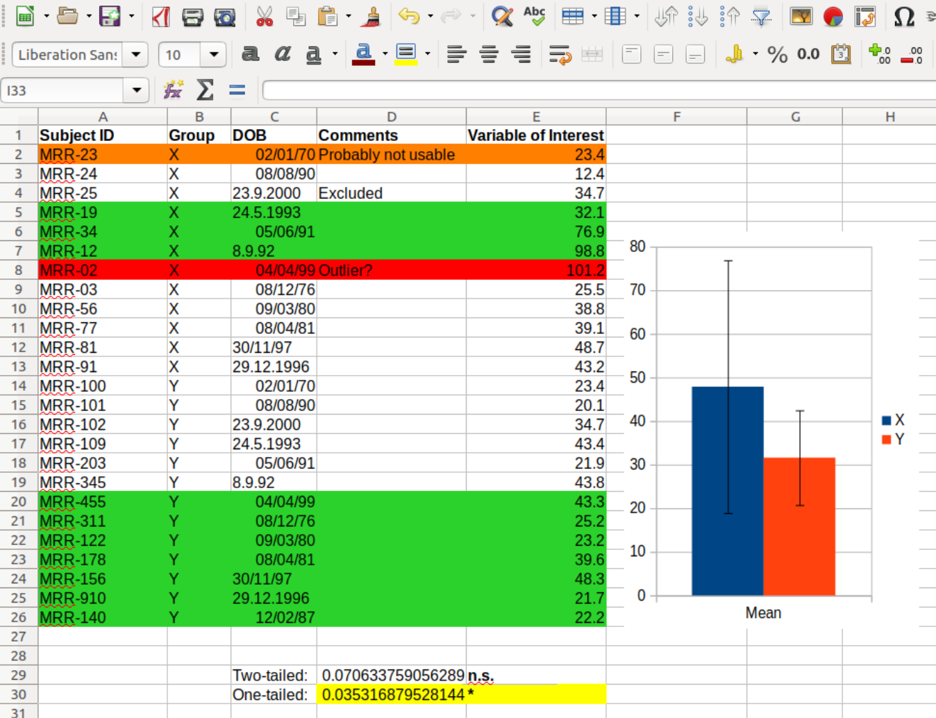
Indeed, I'd argue that not having reproducible work flows is the main reason we often fail at reproducing our own work. We use innocent intuition when organizing data, code, and manuscripts, which may result in excel sheets such as this

where we see some data, quite colorful, together with a dynamite plot and with what appears to be a t-test. So speaking of separating data from code -- was this done here?

The truth is that we are faced with an unhealthy brew of uncleaned data, hidden code, and p-hacked results. The versatility of spreadsheets is cool but it comes at a price, a price that we usually pay a few weeks after compiling such a spreadsheet.

An essential step is thus to strictly separate data from code. This means that once the final data set is compiled (after data cleaning which also wasn't done in the above example) the database is locked, i.e., read-only. Any analysis reads from but never writes to this database. This might seem obvious but I've seen this ignored way too often to be confident it is as obvious as it should be.

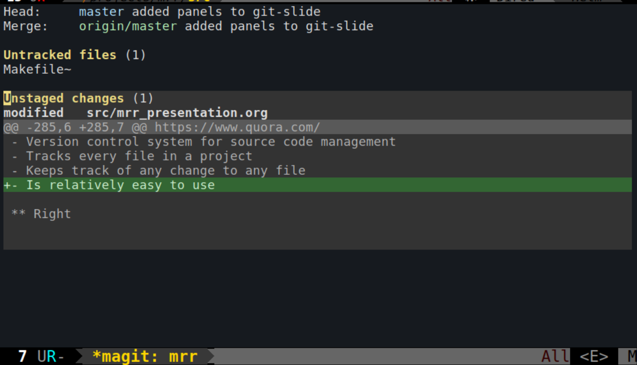
What is version control and why should I use it? For me, this boils down to the quesiton: what is git and why should I use it? Git is a free version control system originally developed to enable to collectively work on the open source operating system Linux. It is in principle a system for source code management, tracking every file in a project and any change therein. It is relatively easy to use but has one downside: it works best with plain text files.

That being said, much of my research work involves writing text, be it code or manuscripts; I even write my presentations and posters in plain text. In a future blog post, I aim to show how scientific manuscripts can ideed be written entirely in plain text, using tools such as emacs or Rstudio. Be that as it may, for computer code, there is really no other option than writing it in plain text. Using a graphical user interfaces (GUIs) such as SPSS or JASP may be appealing to get started but it does have a crucial downside: the workflow is lost after closing the program. What this means is that it will quickly become very difficult to remember the all the steps taken to complete a specific analysis. In other words, it will be difficult to reproduce what we did. Fortunately, the solution is simple: writing computer code to analyze data.

Twitter is full of tweets that celebrate the first successes in writing code. They are all encouraging, and indeed, there is no magic in writing code; once you get started, it's surprisingly simple.

Of course, it is also surprisingly simple to write bad code, sometimes referred to as spaghetti code (not to speak of ravioli code or lasagna code); my early work is full of it (twitter is also famous for examples of people admitting embarrassement about their code, and I'm no exception). Spaghetti code stands for poorly written, hard to maintain computer code; or in other words, computer code that does not make research reproducible. How to avoid it? Here are three rules:

1. Let your variable names speak for themselves
2. Comment your code generously
3. Never write a line of code twice

There is a famous quote that goes like this: There are only two hard things in Computer Science: cache invalidation and naming things (Phil Karlton). Indeed, coding is relatively easy, the real problem is naming variables. Naming variables (and functions) makes your code readable, and style guides (such as this R style guide by google) take it quite seriously. So do spend some time in thinking about reasonable names for variables. Although there is truth to the famous saying that "good code is self-documenting", another recommendation is to be relatively generous with commenting your code. As many have noted, this is mainly a courtesy to your future self who will have much less difficulties understanding your code in the future. Finally, a good rule of thumb is to never write a line of code twice. Whenever you are tempted to do it, you should probably replace it by a function. In fact, you also should not find yourself writing the same function more than once (e.g., across different projects). Instead, put the function into a package; and use the package across projects.

#---------------------------------------------------
# This is a simple R program
# 9/18/18, PH
#---------------------------------------------------
#
# 1. Load and visualize data
#---------------------------------------------------
dat <- read.csv("../data/mrr.csv")

# Histogramms
hist(dat$y[dat$group=="X"], col="blue")
hist(dat$y[dat$group=="Y"], col="blue")

# 2. Compute linear model, adjusted for  age
#---------------------------------------------------
lmfit <- lm(y ~ group + age, data=dat)

# 3. Visualize residuals to check model assumptions
#---------------------------------------------------
plot(density(resid(lmfit)))

# 4. Print coefficients
#---------------------------------------------------
summary(lmfit)

A final remark on organizing code. I mostly use R and python, and have made good experiences with a simple division of labor of my code: one file for all the data cleaning, one for all the functions, one for loading the data, and one for analysing it. Thus, a typical setup for the project myproject would look like this:

• myproject_clean.R
• myproject_load.R
• myproject_func.R
• myproject_do.R

In fact, this setup has been so helpful for me that I decided to write a function that creates it. It is part of the package represearch that I wrote.

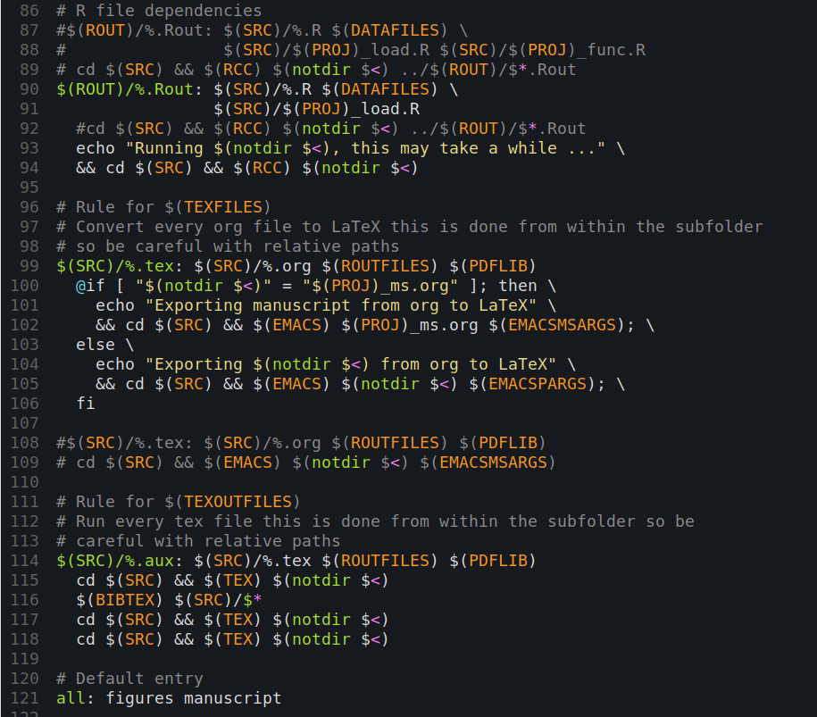
Having written some code to different files, the question arises how to best execute it. Once again, computer scientists have long figured this out. Unix environments include an incredibly powerful command with a name that shines in brevity: make. The command will look for a Makefile in the current directory and will process the commands and dependencies in this file. A Makefile is something like a fancy configuration file for the make command; it can be a little confusing in the beginning.

Yet, a Makefile is just a set of rules that tell make what to do. A Makefile is particularly important when different parts of our code depend on each other. For example, there may be one part that does some sort of preprocessing of the data and another part that runs statistics on that preprocessed data. Now imagine that you found a way to improve the preprocessing -- for example, you realize that it is much better to use the R package readr and its function read_csv() instead of read.csv() to load your comma separated data (see here why this is a good idea). You thus edit your preprocessing file. Ideally, the make routine would notice that your preprocessing file was modified and and that it should be done again. And since the preprocessed data was updated, the statistics on the preprocessed data should also be run again. Indeed, such a rule can be easily set up in the Makefile.

# this is a rule in the Makefile
statistics: preprocessing 
  R CMD BATCH myproj_do.R

# this another rule
preprocessing: datafile1.csv datafile2.csv  
  R CMD BATCH myproj_clean.R

Here, we are telling make that statistics depend on preprocessing, and that preprocessing depends on datafile1 and on datafile2. What this means is that when e.g. datafile2 changes, preprocessing will be run again, that is, the file myproj_preproc.R. And since statistics depend on preprocessing, statistics (that is, the R script myproj_do.R) will also be run in that case.

The benefit of all this may not be obvious for a trivial example where it is easy to keep track what was updated and what needs to be run again. But as soon as our projects start expanding to multiple steps of preprocessing and analysis, such rules are incredibly useful as they free our memory from remembering all the dependencies of our analysis pipeline. We just have to think about them once: when we write the Makefile.

I have argued that making research reproducible requires tools that are well-known in computer science and software development, including version control, Makefiles, and a disciplined coding style.

There are many excellent examples of people reflecting about reproducibility online. The post was inspired by what Jon Zelner wrote about reproducibility, of which I first read about on Andrew Gelman's blog. I would also like to highlight this presentation by Kirstie Whitaker from Cambridge.